CLV Ultra: Our breakthrough new CLV model (and how you can be a part of it)

This article was originally posted by Daniel McCarthy on his LinkedIn page.

Written by Daniel McCarthy, CEO, Theta | January 2024

As those who know me know, I live and breathe CLV modeling, both as an academic and as co-founder of Theta. At Theta, we pride ourselves on developing and implementing the very best methodologies – better than any other commercial provider and better than our award-winning academic work. Over the course of hundreds of engagements, we have refined our CLV model to address myriad issues that we have seen across many companies — incorporating covariates of all shapes and sizes while still being able to run the model almost as quickly as its plain vanilla counterparts; making our model more robust to misspecification; dramatically improving speed and scalability to hundreds of millions of customers (yes, we had an engagement with a company that had hundreds of millions of customers!); better handling of cross-cohort dynamics; and more.

What excites me now is that we’re putting the polish on what I believe will be a truly game-changing CLV model, which we’re endearingly calling CLV Ultra – not only raising the level of our modeling capabilities to new heights, but doing so by leaps and bounds. This work has been led by one of the bright minds on the Theta team, Ian Frankenburg. I’ll share more about the model (and reflections on CLV models more generally) below, and would love to share the model with you more directly — as in, running it on your data — as I’ll discuss more at the end of this post. TLDR: we want to ramp up this model quickly, so as part of that, we are launching a limited pilot program for select companies. You will get CLV estimates for every one of your customers using this model, paying a meaningfully lower price than a normal engagement. In exchange, we will be able to iterate on this model much faster than we otherwise would. Initially, the program will be limited to ensure that the outputs we send to you meet our quality standards, so sign up now! We would love to hear from you if you would like to pilot with us – if so, click here to apply.

About the model

A bit more about the model: we’ve had the opportunity to run it on our own internal equivalent of a “test kitchen,” and have been very happily surprised by its performance. It offers what I believe will be the “best of both worlds” in two ways — (1) higher accuracy with a much higher degree of automation, (2) much easier ability to incorporate covariates with comparable or faster compute time — and easily runs across your entire customer base. It is one of the few cases in which I believe we get to have the proverbial cake and eat it too.

As those who use these sorts of generative CLV models know, this is special because oftentimes, higher accuracy with a given model may require a surprisingly large amount of manual “turning of knobs” — which covariates to include, how exactly to include them, messing with the tuning parameters, etc. This process can be frustratingly laborious. Generative CLV models that allow for covariates are often orders of magnitude slower than their covariate-less counterparts. We have been encouraged that it is computationally cheaper to incorporate covariates (especially individual-level ones) with this new model than with our existing model (which itself was very fast already!).

Generative vs discriminative: Note, above, that I specifically refer to generative CLV models. This is to draw a clear line between the sort of models that we would typically run, and your usual “boosted trees” ML-type model. The latter class of models is discriminative. It cannot generate all of the granular data. Instead, conditional upon your historical data (and that outcome measure of interest, such as 1-year-ahead sales), it can make predictions for other customers based on their historical data.

Discriminative models are not bad in general, but I would argue that they can be bad specifically for the problem of CLV prediction, for a number of notable reasons.

1. You can only include customers for whom you observe the outcome measure of interest. So typically, if you want one-year-ahead sales, you train on all customers with sales over one year as a function of their X’s (at least, this is the de facto norm when someone describes their discriminative CLV model to me). This means that all those customers who aren’t one year old yet are typically ignored. This is a real problem because if there are cross-cohort dynamics, you are kind of flying blind about them as those young customers are not even included in your training data! And remember, the goal of a CLV model is often to predict the value of customers you haven’t acquired yet. Those young customers are going to be the most reflective of the customers you actually care about, so what a shame to have those same customers be the ones who are completely ignored in the model training process.
2. CLV typically entails longer-range projections. And yet, the longer-range your outcome variable, the more data you throw out, because of (1).
3. You can “Franken-model” your way into the longitudinal evolution of spending and other important behaviors of interest (purchases, probability of activity, etc) over time by fitting separate models for different behaviors over different target time horizons. But the resulting collection of predictions need not be internally consistent with one another (e.g., your projections of future purchase counts for a customer may not be consistent with your projections for the probability of activity over a specific time horizon). Your predictions won’t be internally consistent.
4. These models, trained on individual-level data, often do a very poor job at getting the evolution of purchase patterns in aggregate over time. You will often systematically overshoot or undershoot, with the gap getting bigger over time.

Discriminative CLV models thrive on covariates — the more the better! — but I would strongly caution you about the trade-off you are making when considering using these models. For some use cases they are great but for many of the standard CLV use cases they are not.

Visual assessment of model performance

I will provide a few figures that help visually assess the performance of this model on one of the companies we applied it to, which should give you a sense of why I’m so excited. For this company, we did not manually intervene in setting any time-based covariates (although we could if we wanted to). Instead, we simply let our model run across all cohorts jointly. Our hands were off of the proverbial steering wheel, so to speak.

Assessment 1- tracking plots

These are the so-called “tracking plots” for a cohort from this company, with the chart on the left showing week-by-week purchases for the model in both the calibration period (the data that we train the model on), which is to the left of the red dotted line, and the holdout period (the data that we forecast over, which we did not get to train on). The plot on the right is the corresponding “cumulative tracking plot”, representing the cumulative sum of repeat purchases from birth to particular points in time:

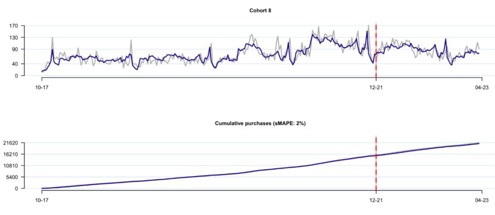
Note: Grey line represents actual data, blue line represents model-based expectation. sMAPE is equal to the symmetric mean absolute percent error off of the cumulative tracking plot over the holdout period, where sMAPE is defined to be \sum_t |A_t – E_t|/(|A_t|+|E_t|), where A_t and E_t are equal to the actual and expected cumulative purchases at time t, respectively.

There is clear evidence of both seasonal variation and more one-off, non-seasonal variation. We do a great job of capturing all the richness in that seasonal variation, which is often hard to do when you are manually specifying covariates. Capturing this richness can be important when you really care what happens next quarter or the quarter after.

Young customers: it also really matters when you want to predict well for young cohorts, who may be affected by that seasonality for the first time, making it hard for the model to know whether that seasonality is indeed seasonality or simply a part of the baseline goodness of the cohort, or relatedly, whether it is a seasonal effect that will recur each year or a non-seasonal effect that will not. The latter issue is just as problematic because in truth, statistical identification of seasonal versus non-seasonal effects is not possible unless you have observed at least two years’ worth of data. At many growing businesses, the vast majority of the active customer base is less than 2 years old, compounding the issue.

What is typically done to account for these issues? Probably the most common solution is to simply pool all the customers who are 2 years or younger together into a single model. The problem with this is that such pooling can often lead to ill-fitting projections when there are cross-cohort dynamics, as it means we’re pooling “apples with oranges.” Separating out these various effects while still allowing young cohorts to be fundamentally different from older ones is a real challenge. And an important one.

This new model can disentangle these various effects — “baseline goodness,” seasonality, non-seasonal shocks, and cross-cohort dynamics — easily, automatically, and interpretably. For visual evidence of this of how well the model fits with young cohorts, check out these tracking plots for a cohort with six months’ worth of calibration period data after the cohort was formed (well less than a year, let alone two), and a 1.25-year holdout period:

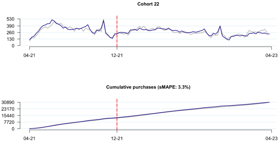
Note: Grey line represents actual data, blue line represents model-based expectation. sMAPE is equal to the symmetric mean absolute percent error off of the cumulative tracking plot over the holdout period, where sMAPE is defined to be \sum_t |A_t – E_t|/(|A_t|+|E_t|), where A_t and E_t are equal to the actual and expected cumulative purchases at time t, respectively.

We didn’t cherry-pick these cohorts. The tracking plots look great, in general, for all of them. We show them all (well, all the incremental tracking plots) below:

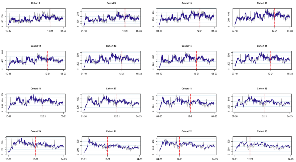
Note: Grey lines represent actual data, blue lines represent model-based expectation.

They also “roll up” into predictions of total purchases across the customer base over time that are remarkably accurate:

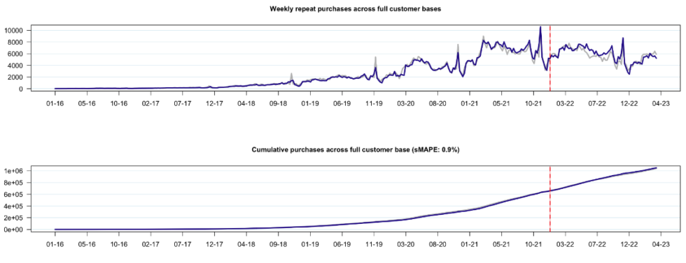
Note: Grey line represents actual data, blue line represents model-based expectation. sMAPE is equal to the symmetric mean absolute percent error off of the cumulative tracking plot over the holdout period, where sMAPE is defined to be \sum_t |A_t – E_t|/(|A_t|+|E_t|), where A_t and E_t are equal to the actual and expected cumulative purchases at time t, respectively.

For customer-based corporate valuation (CBCV) use cases, it is important that we have both accurate predictions at the cohort level, and in terms of overall activity across cohorts. And for marketing use cases, it is important to have accurate predictions at the individual-level and at the cohort level. The figures above showcase just how well-aligned this model is for cohort-level and company-level cases, without any manual model specification whatsoever.

Next, we’ll turn to the individual-level fits.

Assessment 2- conditional expectations

You also get all the usual goodness of a BTYD model in terms of getting “for free” anything else that you may be interested in computing — the probability of activity over different time horizons for different customers, the expected number of purchases for those customers given what you know about them thus far, etc.

One of the ways that we will often assess the goodness of fit of a model at the individual-level is through the so-called “conditional expectations plot”. That is, take all customers that share the same purchase frequency in the calibration period and see how well we can predict what those customers will do over the holdout period.

Here is an example of the CE plot across all existing customers, leaving aside ~16 months as a holdout period:

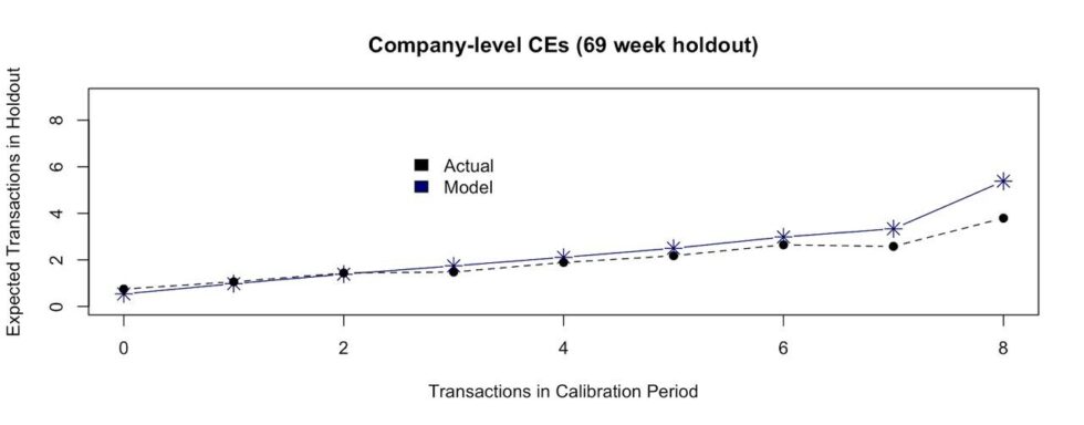
We predict well not only in aggregate within different slices of time, but also when we look at distinct customer segments. And because our model can easily incorporate individual-level covariates, our accuracy can be a lot higher within those customer segments than a traditional BTYD-type of model.

I hope this has left you with a better understanding of what this model can do, and along the way, sparked some thinking about how different types of models, their strengths and weaknesses,  and how to evaluate them.

Join the pilot program!

As mentioned above, we want to get this model up and running quickly. Its combination of accuracy, automation, and speed makes it an even better potential fit for a variety of stakeholders than traditional models — especially companies that have dozens/hundreds/thousands of companies’ data flowing through them. We already have several customers who are advocates and have an open pilot program running currently with positive outcomes. If you’re interested in signing up for the waitlist for a pilot, fill out the CLV Ultra application form.

We want to get the word out far and wide, so would appreciate your help in spreading the good word however you feel comfortable — likes, shares, and/or introductions.

Exciting times!