Probability Modeling: How to Model Customer Churn for a Subscription Business (series)
Written by Hallie Gu, Data Scientist, Theta | October 2022
This is the first post in a series on probability modeling. Throughout the series, we explore the mathematical underpinnings of our Customer-Based Corporate Valuation (CBCV) framework. In this first post, I will focus on customer churn and use a simplified example focused on a subscription business to illustrate the approach. In subsequent posts, we will dive into other aspects of customer behavior and explore various, more nuanced models.
Introduction
Getting the model right is critical when determining the value of a customer base or more importantly, the overall value of your business. Most Customer Lifetime Value (CLV) models, including ours, build on the Buy Till You Die (BTYD) framework, which tells the story of people buying until they become inactive as customers. As the name suggests, a model in the BTYD family includes both repeat purchase and churn components. In this article, I will dive into customer dropoff specifically by walking you through how to model customer churn for a subscription business.

Even though churn in the subscription business is visible and easier to model, most companies still do it wrong. I’ll first show how companies commonly model churn (the wrong approach) then outline a more thorough analysis.
Before we begin, note that the example here is a simplified one to help illustrate the process of probability modeling. Actual churn models are more nuanced and for non-subscription businesses, we would combine churn with the repeat purchasing model (i.e. the complete BTYD model). We’ll cover that in subsequent articles.
Setting up the problem
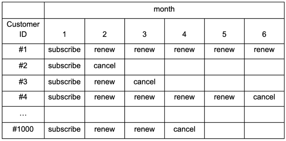
Imagine you are a data scientist at a wine subscription company. Customers sign up to receive one delivery per month and have the option to renew or cancel the subscription at the beginning of each month. We know that 1000 customers subscribed at month one, and the company has the subscription history for all these customers for the first five months.
Your assignment is to predict the number of customers that remain subscribed each month until the end of the year. How would you go about answering the question?
The Data
To start, let’s take a look at the data available. The subscription renewal pattern is as follows:
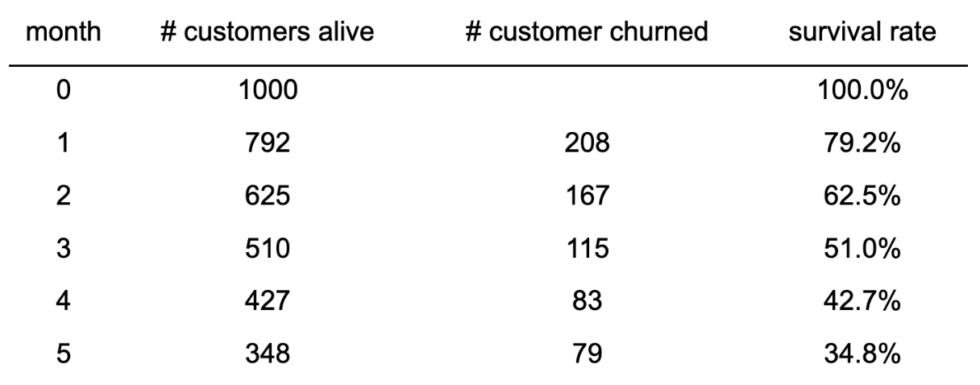
Given the table above, we can calculate the number of customers who “survived” each month as well as the survival rate and retention rate. Note that survival rate (S(t)) is defined as the proportion of the cohort that continues their relationship with the company beyond time t. The survival function is ultimately what we need in order to answer the question at hand.
Model 1: The Wrong Way
To derive a mathematical expression for S(t), we’d need to identify a probability distribution that characterizes a customer’s subscription renewal process. The geometric distribution is an intuitive choice if we make the following assumptions:
- At the start of each month, a customer flips a coin to decide whether to renew (Heads) or cancel (Tails) the subscription
- The monthly coin tosses for renewal decisions are independent from one another
- The probability of churn, p, is constant for every month, and
- All customers have the same propensity to churn
This set of assumptions is very common when companies model churn of their customers. For example, if a customer renews their subscription every month until month three, the results of their three coin tosses are HHT; if a customer renews every month until month four, that means the corresponding coin tosses yielded HHHT. Thus, the probability of a customer canceling at month t can be expressed as P(T= t | p) = p(1-p)t-1 where p is the churn propensity. On the other hand, the probability of a customer “surviving” as of month t, is S(t | p) = (1-p)t.
Now, let’s estimate the churn probability p using Maximum Likelihood Estimation (MLE) on the above data. Let T be the random variable denoting the duration of the customer’s subscription with the firm. Assuming the customer renewal patterns we observe were generated according to the “coin flipping” story, then the likelihood of seeing the observed data (i.e. 208 customers churned after month one, 167 customers churned after month two, … , 348 customers continue subscription as of month five), can be expressed as:

We then estimate parameter p by finding the p value that maximizes the likelihood of seeing the observed data. The estimate for churn propensity turns out to be  = 0.1230, and the plot below shows how well the model-implied survival curve aligns with the actuals.
Of course, the best way to evaluate how good this churn model is, is to test its predictive power in the holdout period (i.e., in the months following our dataset above as shown in the shaded region of the plot).
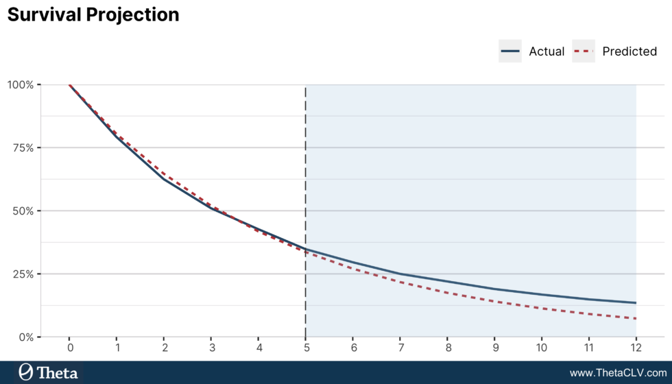
Even though the model does reasonably well in-sample, it significantly underpredicts customer survival for the remainder of the year. To quantify the under-prediction, note that the holdout Mean Absolute Percentage Error (MAPE) is 26.46%. Let’s remember this number, and we will calculate the error for the next model as well for direct comparison. If we use this survival projection to calculate customer lifetime value, we will significantly under-value many customers. How can we do better?
Model 2: The Better Model
Recall that in the previous approach, we assume all customers have the same churn propensity, but in reality, customers are heterogeneous in terms of their subscription renewal behavior. While some customers are die-hard fans of the subscription, others may try it for one month and simply decide they don’t ever want to come back. Therefore, it is very important that we relax assumption #4 from the first model and allow churn probabilities to vary across customers.
…it is very important that we relax assumption #4 from the first model and allow churn probabilities to vary across customers to best model customer churn for a subscription business.
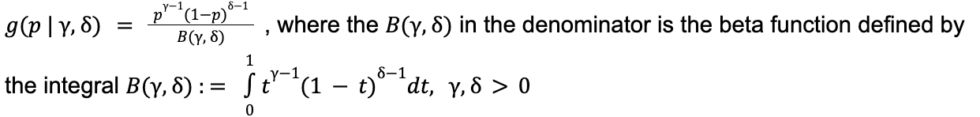
Since each customer’s churn probability is unknown, we will have to treat it as a random variable and specify a probability distribution to characterize how this latent propensity varies across customers. This is called the mixing distribution, and the beta distribution with two parameters  and
and  is a popular choice due to its flexibility and parsimony. In addition, because the beta distribution is defined on the interval [0, 1], it is suitable to represent the distribution of churn probabilities. The expression for the distribution is as follows:
The plot below illustrates the flexibility of the two-parameter beta distribution through the various shapes it can take on. In the context of our business problem, we might be looking at a story where customers are more likely to be either extremely loyal or the complete opposite (bottom left), or another story where the vast majority of the customers have churn probabilities in the 0.1 – 0.4 range (top right). Note that the homogeneous case (constant churn rate across the customer base) is also covered by this approach – it’s just the top right chart with a very narrow distribution and a high spike (when both parameters are significantly larger than 1).

When we combine the geometric distribution at the individual level with the mixing beta distribution at the customer base level, we can derive the so-called beta-geometric distribution:
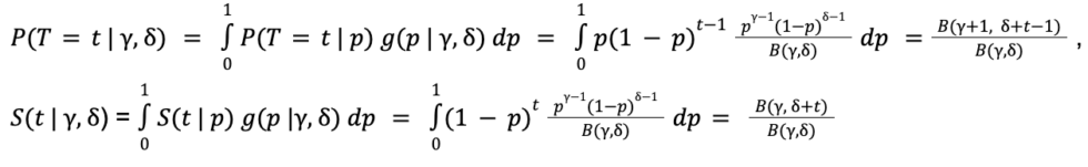
Given the aggregate distribution, we can now express the likelihood of seeing the observed subscription renewal patterns in terms of and (recall that we previously wrote the same expression in terms of p):

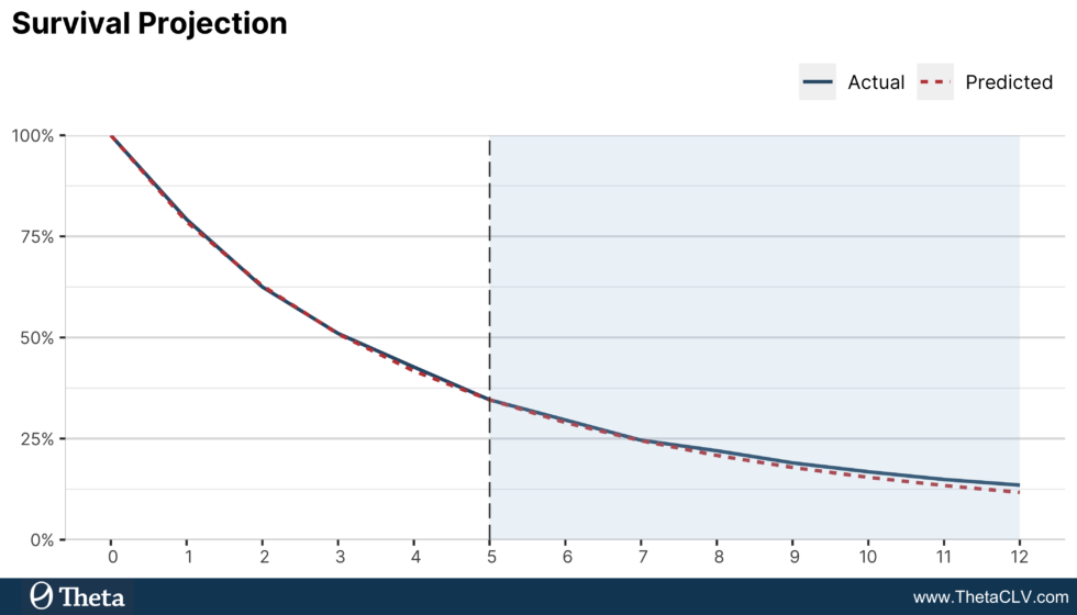
We then find the maximum likelihood estimates for  and
and  which allows us to build the following survival projection. As we can see in the plot, the beta-geometric churn model is able not only to fit the in-sample data better, but also to project survival in the holdout period very accurately, a significant improvement from the geometric model that does not take into account customer heterogeneity. In terms of holdout error, the beta-geometric model yields a MAPE of 6.71%, considerably lower than the 26.46% from the earlier approach.
Conclusion and Next Steps
In the subscription world, companies often use a single churn rate in marketing or finance use cases. However, as we’ve illustrated with the example above, ignoring customer heterogeneity means they will undervalue many customers. Such undervaluation has significant managerial implications. For example, if you knew the true value of customers, you could afford to spend more to acquire them, accelerating company growth; you would also know better which customers to retain and develop, improving profitability. Moreover, undervaluation of customers leads to undervaluation of entire businesses (see what we’ve written before on this topic), which means that companies and their shareholders would leave a lot of money on the table in case of raising capital or sale of the business. The first step is to properly address customer heterogeneity, and the next step is to identify and focus on the high value customers for long-term success.
This article is an introduction to the customer behavior models that laid the foundation for the work we do at Theta. In subsequent articles, we will discuss other commonly used churn models in non-subscription settings, as well as expand our conversations to repeat purchase and spend behaviors, the other two components of a complete customer behavior analysis.